Dreamer V3

A brief introduction

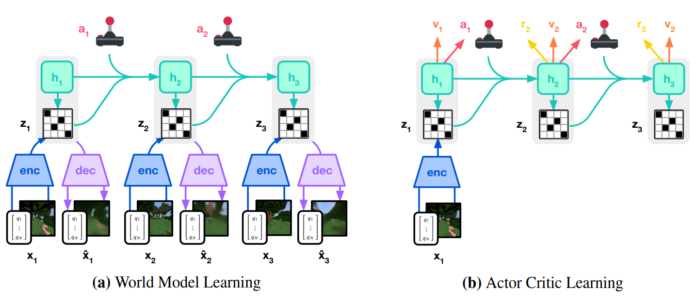
It is time for the last (maybe) Dreamer implementation, we are talking about DreamerV3, the SoTA RL algorithm released in January 2023 by Hafner et al. [1]. This algorithm enables to solve tasks across several domains with fixed hyperparameters. As its predecessors, Dreamer-V3 is an off-policy agent (i.e., it can learn the optimal policy from a different policy), and a model-based algorithm, meaning that it learns the dynamics of the enviromnet by creating a latent representation of the world and exploit this latent representation to imagine consequences of it actions. To know how the algorithm works, please have a look of our Dreamer-V1 [2] and Dreamer-V2 [3] blogposts. In Figure 1 a general and high level rappresentation of how the models of Dreamer-V3 works. In Figures 3, 4 and 5 are shown some results about Dreamer-V3, trained on the MsPacman environment in 100K steps.

Figure 1: An overview over DreamerV3 models [1]. The world model (a) learns the dynamics of the environment (dynamic learning). The encoder compute the observations embeddings, that are used by the RSSM to compute the latent states (composed by $h_t$ and $z_t$). Moreover, the agent learns to estimate the rewards, the dones and to reconstruct the observations from the latent states. Instead, in the behaviour learning (b), the agent imagines the consequences of its actions to learn the optimal behaviour.

In the next section the differences between Dreamer-V2 and Dreamer-V3 will be described. There are not significant differences in the main idea of the algorithm, but there are a lot of little details that are changed and that significantly improved the performance.

Dreamer-V3 vs Dreamer-V2

We are now going to list the differences between Dreamer-V3 and its predecessor. As anticipated before, the components of the two agents are the same (as the ones employed in Dreamer-V1), thus we will not go into detail about the componets of the agent (refer to our Dreamer-V1 post to have a detailed introduction on every Dreamer components’). The only thing to note here is that the continue model predicts the continues (whether or not the episode continues), insetad of predicting the probability of likelihood of continuing the episode as done in Dreamer-V2.

Symlog predictions

Figure 2: The symlog function. It compresses the magnitudes of both large positive and negative values, allowing to quickly move the network predictions to large values when needed.

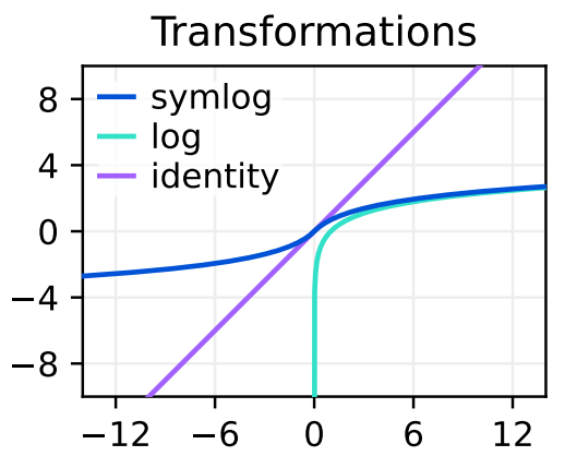
As mentioned before, Dreamer-V3 aims to solve tasks in different domains, a difficult challenge because of the varying scales of inputs, rewards and values. To solve this issue, Hafner et al. propose to use symlog predictions, i.e., given a neural network $f(x, \theta)$, with inputs $x$ and parameters $\theta$, learns to predicted the symlog transformed targets: $\mathcal{L}(\theta) \doteq \frac{1}{2}\left( f(x, \theta) - \text{symlog}(y) \right)^2$. Where the symlog function is defined as follows:

Given the neural network prediction, it is possible to obtain the non-transformed target by appling the inverse transformation (i.e., the symexp):

The last detail to report is that the symlog prediction is used in the decoder, the reward model and the critic. Moreover, the inputs of the MLP encoder (the one that encodes observations in vector form) are squashed with the symlog function (Figure 2).

KL regularizer

As in Dreamer-V2, during the dynamic learning phase, the posterior and the prior (estimated by the representation and the transition models, respectively) are learned to minimize their KL divergence. Since, 3D domains may contain unnecessary details whereas in 2D domains the background is often static and each pixel could be important for solving the task, the KL loss was slightly modified. The KL loss is divided in two losses: the dynamic and the representation.

The dynamic loss is the follwing: \(\mathcal{L}_{\text{dyn}}(\phi) \doteq \max\left(1, \text{KL}(\text{sg}(P) \Vert Q) \right)\)

The representation loss is the following: \(\mathcal{L}_{\text{rep}}(\phi) \doteq \max\left(1, \text{KL}(P \Vert \text{sg}(Q)) \right)\)

Where $1$ is the free bits used to clip the dynamic and representation losses below of the free bits, necessary to avoid degenerate solutions where the dynamics are trivial to predict, but do not contain enough information about the inputs. Finally, to have a good balance between complex and very detailed environments (e.g, 3D envs) and simpler and less detailed environments (e.g., static 2D envs), the two losses are scaled differently and summed together.

Uniform Mix

To prevent spikes in the KL loss, the categorical distributions (the one for discrete actions and the one for the posteriors/priors) are parametrized as mixtures of $1\%$ uniform and $99\%$ neural network output. This avoid the distributions to become near deterministic. To implement the uniform mix, we applied the uniform mix function to the logits returned by the neural networks.

import torch
from torch import Tensor
from torch.distributions.utils import probs_to_logits

def uniform_mix(self, logits: Tensor, unimix: float = 0.01) -> Tensor:
    if unimix > 0.0:
        # compute probs from the logits
        probs = logits.softmax(dim=-1)
        # compute uniform probs
        uniform = torch.ones_like(probs) / probs.shape[-1]
        # mix the NN probs with the uniform probs
        probs = (1 - unimix) * probs + unimix * uniform
        # compute the new logits
        logits = probs_to_logits(probs)
    return logits

Return regularizer for the policy

The main difficulty in Dreamer-V2 actor learning phase is the choosing of the entropy regularizer, which heavily depends on the scale and the frequency of the rewards. To have a single entropy coefficient, it is necessary to normalize the returns using moving statistics. In particular, they found out that it is more convenient to scale down large rewards and not scale up small rewards, to avoid adding noise.

Moreover, the rewards are normalized by an exponentially decaying average of the range from their $5^{\text{th}}$ to their $95^{\text{th}}$ percentile. The final actor loss becomes:

Where $R^{\lambda}_{t}$ are the returns, $a_t$ is the action, $s_t$ is the latent state ($z_t$ and $h_t$ of Figure 1), and

Critic learning

As in Dreamer-V2, there are two critics: the critic and a target critic (updated with an exponential moving average at each gradient step). Differently from V2, in Dreamer-V3, the lambda values (the returns) are computed with the values estimated by the critic and not the values estimated by the target critic. Moreover, the critic is trained to correctly estimate both the discounted returns the target critic predictions.

Another difference is that the critc learn the twohot-encoded symlog-transformed returns, to be able to predict the expected value of a widespread return distribution. So, the symlog-transformed returns are discretized into a sequence of $K = 255$ equally spaced buckets, whereas the critc outputs a softmax distribution over the buckets.

The twohot encoding is defined as follows:

Where $x$ is the input to encode, $i$ is the index of the twohot, $b_k$ is the value of the $k$-th bucket and $k = \sum^{B}_{j=1}\delta(b_j \lt x)$.

In this way a nuber $x$ is represented by a vector of $K$ numbers, all set to zero except for the two positions corresponding to the two buckets among which is situated $x$. For instance, if you have $5$ buckets which equally divide the range $[0, 10]$ (i.e., the $5$ buckets are: $[0, 2.5, 5, 7.5, 10]$) and you have to represent the number $x = 5.5$, then its two hot encoding is the following:

Because $5.5$ is closer to bucket $5$ than bucket $7.5$.

Models

The last differences concern the hyperparameter used, for instance, the used activation function is the SiLU. Moreover, all the models use the LayerNorm on the last dimension, except for the convolutional layers that apply the layer norm only on the channels dimension. The last detail is the presence of the bias in the models, in particular, all the layers followed by a LayerNorm are instantiated without the bias.

Implementation

Our PyTorch implementation tries to faithfully follow the original TensorFlow implementation, aiming to make the code clearer, scalable and well-documented. We used the same weight initialization of the models: all the models are initialized with a xavier normal initialization [4], except for the heads of the actor, the last layer of the transition, representation, continue and encoder models that are initialized with a xavier uniform initialization [4] and the last layer of the critic and the reward model that are initialized with all zeros (to speed up the convergence).

Finally, the last difference with Dreamer-V2 is how experiences are stored in the buffer: in Dreamer-V2 each action was associated to the next observations, instead in Dreamer-V3, the actions are associated to the observations that have led the agent to choose that actions, so in Dreamer-V2 an action was associated to its consequences, instead in Dreamer-V3 the observation is associated to the next action to be performed.

Do you want to know more about how we implemented Dreamer-V3? Check out our implementation.

Results

References