Dreamer V2

Dreaming with a discrete world-model

In this blogpost we are going to introduce Dreamer-V2 [2], the natural extension to the already covered DreamerV1 [1] algorithm. As its predecessor, Dreamer-V2 is both an off-policy and a model-based algorithm, where the former means that it learns from previous experiences gathered with a different policy than the one the agent is trying to learn, while the latter means that is capable of learning long-horizon behaviours purely by latent imagination, i.e. it learns an embedded representation of the real environment and uses this embedded representation to learn the optimal policy. For a detailed introduction to the generalities of the algorithm please have a look at our previous blogpost.

Figure 1: An overview over DreamerV2 World-Model [2]. The training sequence of images $x_t$ is encoded using the CNN. The RSSM uses a sequence of deterministic recurrent states $h_t$. At each step, it computes a posterior stochastic state $z_t$ that incorporates information about the current image $x_t$, as well as a prior stochastic state $\hat{z}_t$ that tries to predict the posterior without access to the current image. Unlike Dreamer-V1, the stochastic state of Dreamer-V2 is a vector of multiple categorical variables.

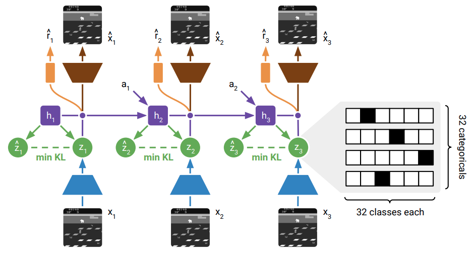
One of the main differences with respect to the first version is that Dreamer-V2 learns a discrete latent state of the environment as a mixture of 32 categoricals with 32 classes each. This discretization of the latent state is helpful for different reasons (as stated directly by the authors):

• A categorical prior can perfectly fit the aggregate posterior, because a mixture of categoricals is again a categorical. In contrast, a Gaussian prior cannot match a mixture of Gaussian posteriors, which could make it difficult to predict multi-modal changes between one image and the next.
• The level of sparsity enforced by a vector of categorical latent variables could be beneficial for generalization. Flattening the sample from the 32 categorical with 32 classes each results in a sparse binary vector of length 1024 with 32 active bits.
• Despite common intuition, categorical variables may be easier to optimize than Gaussian variables, possibly because the straight-through gradient estimator [1] ignores a term that would otherwise scale the gradient. This could reduce exploding and vanishing gradients.
• Categorical variables could be a better inductive bias than unimodal continuous latent variables for modeling the non-smooth aspects of Atari games, such as when entering a new room, or when collected items or defeated enemies disappear from the image

Dreamer-V1 vs Dreamer-V2

We are now going to list the differences between Dreamer-V2 and its predecessor. Since the model components are exactly the same as the ones employed in Dreamer-V1, those will be skipped (refer to our previous post to have a detailed introduction on every Dreamer components’). The only thing to note here is that the model is bigger w.r.t. the number of parameters: increasing the number of dense units in the MLPs or feature maps per layer of all model components resulted in a change from 13M parameters to 22M parameters.

KL balancing

During the dynamic learning phase, i.e. the one in which the world model is learned, the prior distribution over the latent states, estimated by the transition model, and the posterior one, estimated by the representation model, are learned so to minimize their KL divergence:

where $P,Q,\text{H}(P,Q)$ and $\text{H}(P)$ are the posterior and prior distributions, the cross-entropy between the posterior and the prior and the entropy of the posterior distribution respectively. The KL loss serves two purposes: it trains the prior toward the representations, and it regularizes the representations toward the prior. However, since learning the prior is difficult, we want to avoid regularizing the representations toward a poorly trained prior. To overcome this issue, the divergence between the posterior and the prior is replaced with the following:

with $\alpha = 0.8$ and $\text{sg}$ stands for “stop-gradient” ($\texttt{.detach()}$ on a PyTorch tensor). By scaling up the prior cross entropy relative to the posterior entropy, the world model is encouraged to minimize the KL by improving its prior dynamics toward the more informed posteriors, as opposed to reducing the KL by increasing the posterior entropy.

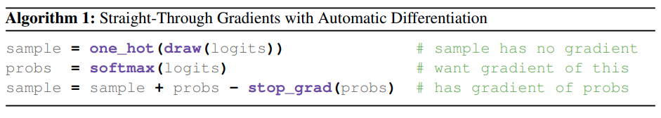
Straight-Through gradients

The Straight-Through gradients trick let us backpropagate through a drawn sample from a Categorical distribution: this lets the world model to receive gradients from both the KL balancing loss and the sampled latent states, subsequently used to estimate rewards, reconstruct the observations and predict the continue flag.

Figure 2: The Straight-Through Gradients [3].

Policy gradient and the actor loss

DreamerV1 relied entirely on reparameterization gradients to train the actor directly by backpropagating value gradients through the sequence of sampled model states and actions. DreamerV2 uses both discrete latents and discrete action and to backpropagate through the sampled actions and state sequences straight-through gradients are leveraged. This results in a combined actor loss function like the following:

where:

• \(-\ln p_\psi(\hat{a}_t\vert\hat{z}_t)\text{sg}(V_t^\lambda - v_\xi(\hat{z}_t))\) is the reinforce term, which aims to maximize the actor’s probability of its own sampled actions weighted by the values of those actions. The benefit of Reinforce is that it produced unbiased gradients and the downside is that it can have high variance.
• $-V_t^\lambda$ is the dynamics term, which aims to output actions that maximize the prediction of long-term future rewards made by the critic. Thanks to straight-through gradients we can backpropagate through the sampled actions and state sequences. This results in a biased gradient estimate with low variance.
• $-\eta\text{H}[\hat{a}_t\vert\hat{z}_t]$ is the entropy term, which favors a more explorative policy by increasing its entropy.

Even though annealing the $\rho$ hyperparameter could lead to a better solution (the low-variance but biased dynamics backpropagation could learn faster initially and the unbiased but high-variance could to converge to a better solution later on during the training), the authors have set it to $\rho=1$ for discrete environments, while to $\rho=0$ for continuous one.

The policy used for the actor is a Truncated Normal distribution, for which a PyTorch implementation can be found here.

Implementation

Our PyTorch implementation aims to be a simple, scalable and well-documented replica of the original TF2 implementation. To demonstrate the effectiveness of our implementation we trained Dreamer-V2 on both the Atari Pong and the DMC Walker-Walk with the standard hyperparameters suggested by the authors for continuous and discrete environments. Some qualitative results are showed at the beginning of the post.

As an example, the implementation of the KL balancing directly follows the equation above:

from torch.distributions import Independent, OneHotCategoricalStraightThrough


lhs = kl_divergence(
    Independent(OneHotCategoricalStraightThrough(logits=posteriors_logits.detach()), 1),
    Independent(OneHotCategoricalStraightThrough(logits=priors_logits), 1),
)
rhs = kl_divergence(
    Independent(OneHotCategoricalStraightThrough(logits=posteriors_logits), 1),
    Independent(OneHotCategoricalStraightThrough(logits=priors_logits.detach()), 1),
)
kl_loss = alpha * lhs + (1 - alpha) * rhs

Do you want to know more about how we implemented Dreamer-V2? Check out our implementation.

References