Dreamer V1

Behind our PyTorch implementation of the State-of-the-Art RL algorithm.

With the exponential growth of deep learning and computational power, RL algorithms have evolved significantly and model-based algorithms have become increasingly popular in recent years. A model-based algorithm aims to learn the dynamics of the environment and exploits them to properly select the best option. DreamerV1 [1] is a model-based approach, capable of learning long-horizon behaviours from images purely by latent imagination, meaning that it learns an embedded representation of the real environment and uses this embedded representation to learn the optimal policy. Moreover, it is an off-policy algorithm, so it learns from previous experiences gathered with a different policy than the one the agent is trying to learn.

Since its publication, Dreamer has attracted much interest in the RL world because of the revolutionary idea behind it and its impressive performance, but because of its complexity, there are few implementations and not so easy to understand. For this reason, we have meticulously studied DreamerV1 and its original implementation in Keras/Tensorflow, to provide a reliable, efficient, and easy to understand version in PyTorch. Check out our implementation.

A Look inside Dreamer

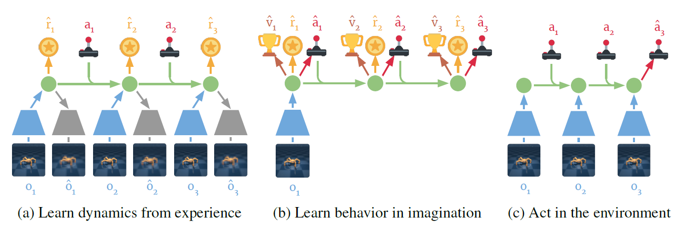
Let’s start getting familiar with Dreamer: as mentioned before, it can abstract observations to predict rewards, values, and to select actions; leveraging on a smaller memory footprint than predictions in image space, allowing Dreamer to image thousands of trajectories in parallel (Figure 1). Each latent state is made by two parts: a deterministic part, henceforth called recurrent state, which embeds all the history of the episode; and a part called stochastic state, that embeds more information about the actual state (i.e, the real state the agent is currently in).

Figure 1: An overview over DreamerV1 [1]. *(a)* The World model learns the dynamics of the environment. *(b)* Then Dreamer learns to behave only from latent imagination. Finally, *(c)* the agent exploits what it have learned to act in the environment.

Components

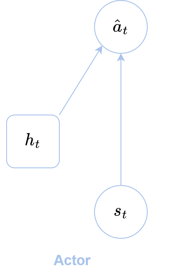
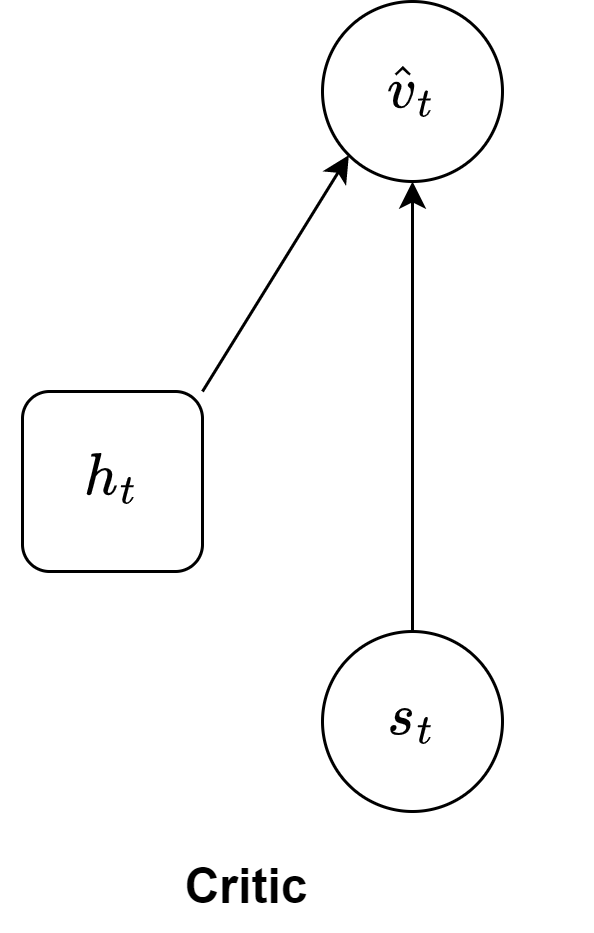
As one can imagine, Dreamer is a complex agent which is made of various components: a world model, an actor and a critic. The first one is responsible to learn the latent representation of the environment; the actor selects the actions from the latent state; whereas the latter component predicts the state values from the computed latent states.

The world model is the most complex and it is composed by five parts. (i) An encoder, that is a fully convolutional neural network, encodes the pixel-based observations provided by the environment. (ii) An RSSM (Recurrent State-Space Model [2]) which generates the latent states, and it is composed by three models:

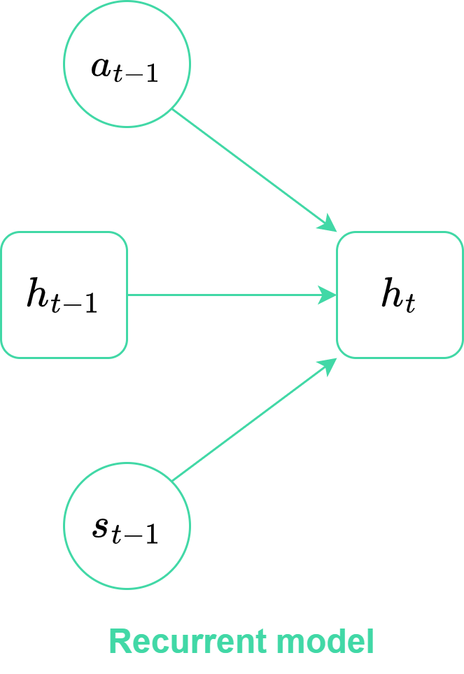
1. The recurrent model: a linear layer followed by an ELU activation function and a GRU, that encodes the history of the episode and computes the recurrent state.
2. The representation model: an MLP, that computes the stochastic state from the recurrent state and the actual observations.
3. The transition model: an MLP, that predicts the stochastic state given only the recurrent state, it is used to imagine trajectories in the latent dynamic.

Additionaly, (iii) there is an observation model consisting of a linear layer followed by a convolutional neural network with transposed convolutions; this reconstructs the original observation from the latent state. Then, (iv) a reward model (MLP) predicts the reward for a given latent state. Finally, (v) an optional continue model (MLP) estimates the discount factor of the TD($\lambda$) values.

Implementation

Now that we have a general overview of how Dreamer works, we can dwell on all the details of this algorithm. First, it is necessary to shed light on the learning algorithm, which is divided in two parts: in the first one the agent learns the latent representation (dynamic learning), whereas in the second it learns the actor and the critic while the world model is frozen (behaviour learning).

Dynamic Learning

In this phase the agent learns a latent representation of the environment from a batch of sequences, The key component of the world model is the RSSM, that embeds the environment states into latent states. As mentioned before, the latent state consists of a recurrent state, encoding the episode’s history, and a stochastic state containing additional information about the current state (i.e, the state the agent is currently in). The recurrent model, implemented as a dense layer followed by a GRU, is responsible for embedding the history of the sequence and computing the recurrent state (ht in Figure 2) from the previous action, recurrent state and stochastic state.

Figure 2: How the models of the RSSM works. The recurrent model encodes the history of the episode. The representation model tries to encode the consequences of the performed action, so what is happening. The transition model tries to imagine what will happen.

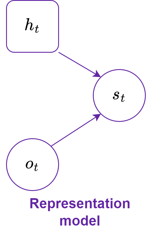
The representation model and the transition model both compute the distribution of the stochastic state ($p$ and $q$, respectively), but the former uses observations (encoded by the encoder), whereas the latter does not; then the stocastic state is sampled from these distributions. So, the representation model uses the observations (embedded by the encoder) to compute the stochastic state, whereas the transition model does not use it. This means that the recurrent model is more precise than the transition model, but the transition model is crucial for imagining trajectories in the latent space (which is more efficient and less computationally expensive than doing so in image space).

Figure 3: How the RSSM works. The three models of the RSSM iteratively compute the recurrent and stochastic state.

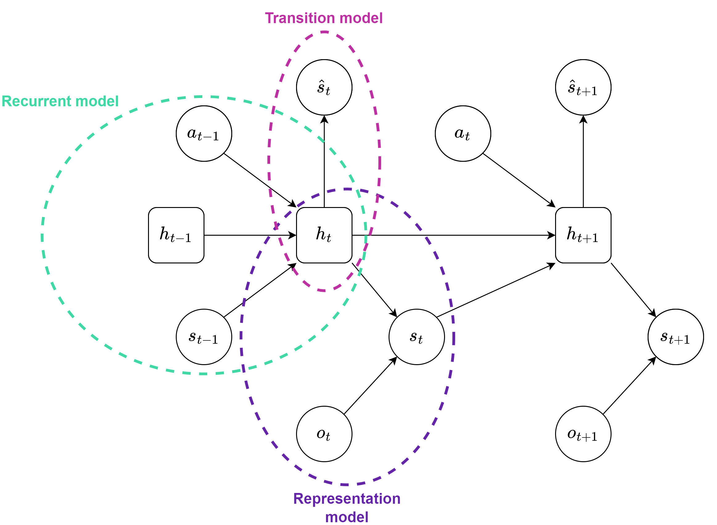
The states, computed by the RSSM (Figure 3), must be reliable and consistent with the environment in order for the agent to predict rewards, values, discounts of the values and, select actions. To achieve this, the reward model and continue model learn to predict rewards and discounts (the probability that the episode has ended at a specific time step), respectively; moreover, the observation model aims to reconstruct the environment observations from the latent states.

Following what Hafner et al wrote in the paper [1], the data for a single gradient step is organized into a batch of 50 sequences, each with a length of 50. The dimensions of the data depend on the type of data, e.g., RGB observations have sizes equal to (3, 64, 64). The observations are scaled to the range of [-0.5, 0.5] to facilitate easier reconstruction by the observation model. The proper initialization of states for the recurrent model is crucial: both the recurrent state and stochastic state are initialized as tensors of zeros. The core part of dynamic learning involves computing all the latent states. A for loop is necessary because of the structure of the RSSM, in which the recurrent unit takes as input the previous action and latent state.

After computing all the latent states in the batch, the next steps involve learning to reconstruct the original observations and predict rewards, as well as computing the probability of episode continuation from the computed latent states. The reward and observation models provide mean predictions for the reward and observation normal distributions ($q_r$ and $q_o$ respectively), while the continue model outputs logits of a Bernoulli distribution ($q_c$). These predictions are compared with the real information provided by the environment: the world model loss, also known as the reconstruction loss, is computed as follows:

Where $\hat{d} \sim q_c $, and $d$ are the dones received by the environment.

Behaviour Learning

After completing the dynamic learning phase, the next step is to learn the actor and critic using the learned world model. The objective is to use the world model to imagine the consequences of actions. The imagination process starts from a real latent state, computed from the representation model, and continues for a certain number of imagination steps (horizon). During each step, the agent selects an action based on the current latent state (actor in Figure 3) and computes the next latent state using the world model.

Figure 3: How the actor works. It selects the action from the lantent state (recurrent and stochastic state).

The recurrent and transition models of the RSSM, as shown in the Figure 4, are used for imagining trajectories. The transition model is employed instead of the representation model because the environment observations are not available during imagination. Additionally, imagining in the latent space is faster and more cost-effective than doing so in the image space, making the transition model more convenient.

Figure 4: Imagination phase. The actor, the recurrent and the transition models iteratively perform the imagination steps. The actor comptes the next actions, then the recurrent model encodes this information in the recurrent state. Finally the transition model predicts the stochastic state.

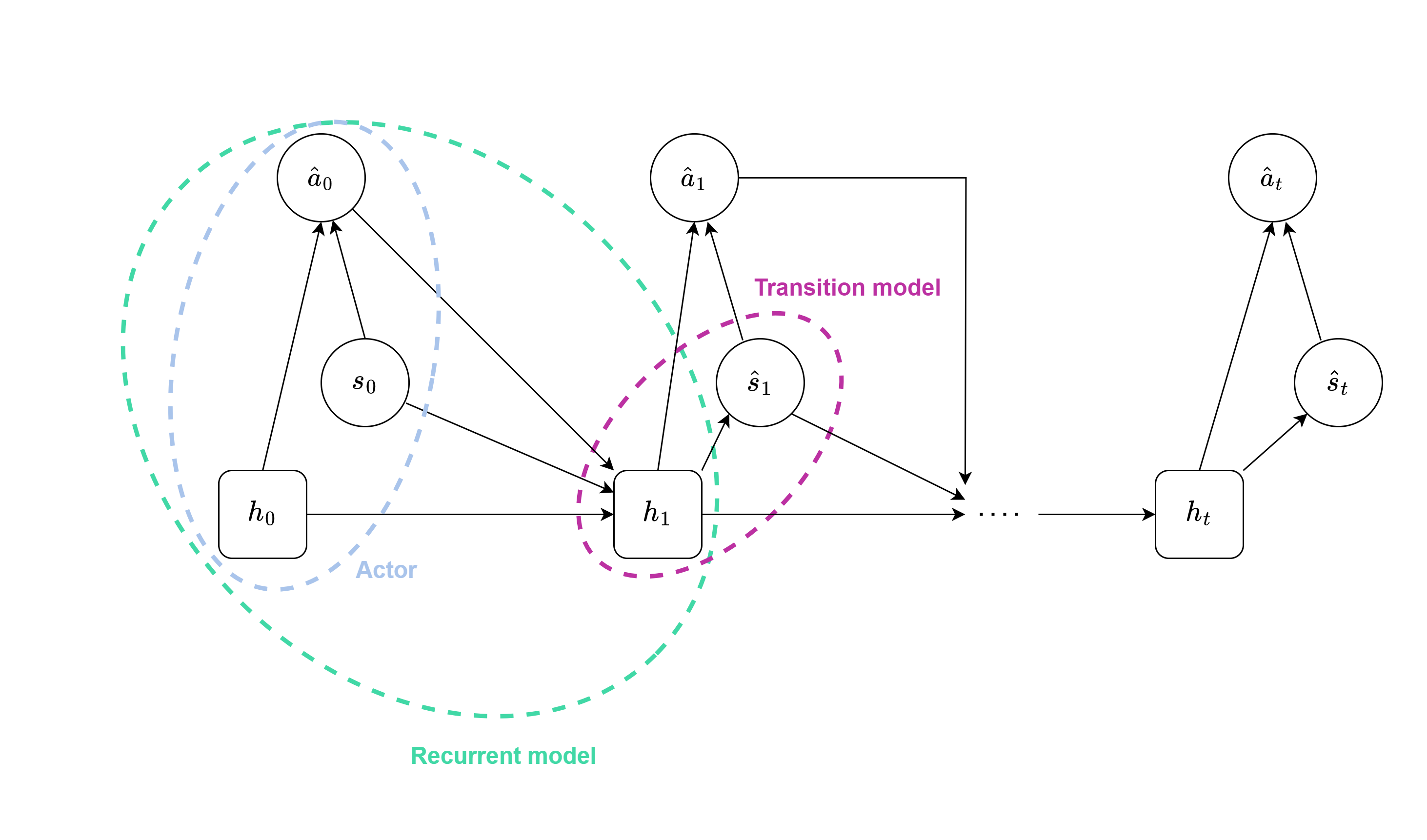
All the latent states computed in the previous phase (dynamic learning) serve as starting points for fully imagined trajectories. Consequently, the latent states are reshaped to consider each computed latent state independently. A for loop is necessary for behavior learning, as trajectories are imagined one step at a time. The actor selects an action based on the last imagined state, and the new imagined latent state is computed.
From the imagined trajectories, the critic (Figure 5), reward model, and continue model predict values, rewards, and continue probabilities, respectively. These predicted quantities are used to compute the lambda values (TD($\lambda$)), which serve as target values for actor and critic losses.

Figure 5: How the critic works. It estimates the state value from the lantent state (recurrent and stochastic state).

An important consideration is the composition of the imagined trajectories. The starting latent state computed by the representation model (from the recurrent state and embedded observations) must be excluded from the trajectory because it is not consistent with the rest of the trajectory. This was one of the initial challenges faced during the implementation of Dreamer, and without this adjustment, the agent would not converge.

When computing the lambda values, the last element in the trajectory is “lost” because the next value is needed to calculate the TD($\lambda$), but the last imagined state does not have a next value. Moreover, according to the DreamerV1 paper, the lambda targets are weighted by the cumulative product of predicted discount factors ($\boldsymbol{\gamma}$), estimated by the continue model. This weighting downweights terms based on the likelihood of the imagined trajectory ending. This crucial detail, necessary for convergence. These weighted lambda targets are used in the actor loss as part of the update process. Instead, the critic predicts the distribution of the values ($q_v$) without the last element of the imagined trajectory and then it is compared with the lambda values. The actor and critic losses are computed as follows:

Actor

The actor ($a$) of Dreamer supports both continuous and discrete control. For continuous actions, it outputs the mean and standard deviation of the actions. The mean is scaled by a factor of 5, and the standard deviation is processed using a SoftPlus function to ensure non-negative values. The formulas for calculating the mean and standard deviation are not explicitly described in the paper, but can be derived from the code. The standard deviation is increased by a raw init std value and then transformed using SoftPlus, with a minimum amount of standard deviation added to the result. The resulting normal distribution is transformed using a hyperbolic tangent (tanh) function, and the Independent distribution is used to set the correct event shape. The mean and standard deviation for the discrete control are computed as follows:

Where $\chi = \ln e^{5 - 1}$ is the raw init std value and $\mu_{\phi}$ and $\sigma_{\phi}$ are the mean and standard deviation computed by the actor.

In the case of discrete actions, no transformations are applied to the model output, which serves as the logits of a one-hot categorical distribution. The actor can be used in both training and test modes. In training mode, it produces a sample with gradients as output, while in test mode, it selects the best possible actions for a given state. For continuous control, a sample with gradients is obtained using reparameterization sampling, and the best possible action according to the learned policy is given by the mode of the distribution of the actions. In the case of discrete actions, straight-through gradients are used for sampling during latent imagination, and the mode of the one-hot categorical distribution is used to select the best possible action during test.

Environment Interaction

The environment interaction in Dreamer involves the agent selecting actions, receiving rewards and observations from the environment. There are two types of interaction: one during training with noisy actions for exploration and episodes saved in the replay buffer, and another where the agent plays optimally based on the learned policy.

Since the agent operates entirely in the latent space, several models are needed: the encoder to encode observations, the recurrent model to compute the recurrent state, the representation model to compute the stochastic state, and the actor to select actions from the latent states. The environment interaction follows the standard RL approach: the agent starts from an initial observation, selects actions, and receives information from the environment such as next observations, rewards, done (indicating episode termination), truncated (indicating episode cutoff), and additional information; moreovere it keeps track of the previous lantent state and previous action (initialized to tensors of zeros). If done or truncated is true, the agent resets its state, and a new episode starts (in training mode the episode is added to the buffer, associating the action to the next observation, the reward and the done or truncated).

To improve performance, some expedients can be applied. These include action repeat, where an action is repeated multiple times, and limiting the maximum number of steps in an episode to encourage exploration. Other hyperparameters include reward clipping, using grayscale instead of RGB images, and setting a maximum number of no-ops in Atari environments. Furthermore, it can be useful to collect some episodes with random actions before training, as the agent is an off-policy algorithm and can learn from experiences gathered with a different policy.

Sequential Replay Buffer

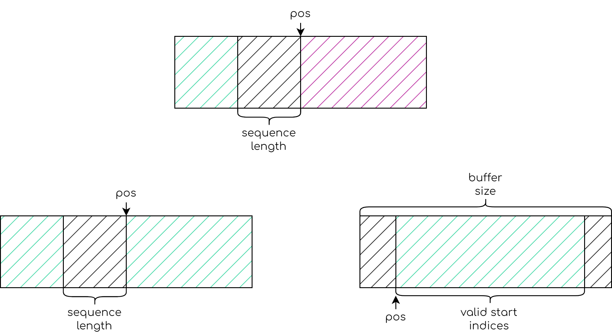
To properly save and retrieve experiences, Dreamer uses a sequential replay buffer with a custom sample function. The sample function randomly selects a batch of starting indices for the sequences. From these starting indices, all the indices of the corresponding sequences are computed, and the data is retrieved from the buffer.

If the buffer is not full, the starting indices can be sampled from zero to the index of the last filled cell in the buffer minus the sequence length ($\text{sl}$) (i.e., $\text{pos}- (\text{sl} - 1)$). However, if the buffer is full and older experiences are being replaced, the starting indices cannot fall between $\text{pos} - \text{sl}$ and $\text{pos}-1$. If $\text{pos} - \text{sl}$ is negative, it indicates the need to circularly go back in the buffer and remove positions from the bottom (Figure 6).

Figure 6: Possible cases of buffer sampling: above is the case where the buffer is not full, and below are the two cases with full buffer. In green the valid starting indices; in grey the indices that can be sampled, but not as starting indices; in red the indices that cannot be sampled.

Critical Aspects

To ensure convergence of the algorithm, several significant details were identified. Firstly, it was found that reducing the dimension of the models to speed up training and save memory did not yield satisfactory results. Moreover, the GRU (Gated Recurrent Unit) was determined to be the most effective recurrent unit for the recurrent model, and processing the entire sequence at once was not feasible.

The choice of activation functions was found to have a considerable impact on performance. It is recommended to use the specified activation functions in the paper and to be careful whether or not the activation should be applied after the last layer of the neural network, e.g., the ReLU activation function must be applied after the last convolutional layer in the encoder, but not after the last layer of the observation model.

Properly using distributions and handling model outputs were also crucial. The action distribution and the stochastic state distribution were sensitive to changes in hyperparameters. All distributions used in the algorithm are Normal distributions, except for the distribution estimating the probability of episode termination, which is a Bernoulli distribution. Paying attention to the batch shape and event shape of the distributions is crucial. For example, the reconstructed observation distribution should have a batch shape of $(\text{sequence_length}, \text{batch_size})$ and an event shape of $(C, H, W)$.

In the training process, two key aspects were important: removing the initial state from the imagined trajectory (computed by the representation model) and introducing the cumulative product of discounts computed from the probabilities of episode termination (estimated by the continue model). Finally, the breakthrough in the algorithm’s performance was achieved through proper environment interaction and the use of a buffer. Observations were normalized to the range [-0.5, 0.5]. The action was associated with the next observations, and the initial observations were associated with an all-zero action.

Results

Our implementation aimed to replicate the well-known and well-documented results of DreamerV1. One of the key features of Dreamer is its ability to simulate the outcomes of actions. To demonstrate the effectiveness of our implementation, we trained Dreamer on Ms. Pacman for 5.000.000 steps, using an action repeat of 2 and a maximum episode length of 1000. We closely observed the behavior of the agent and analyzed its capacity to imagine future states. The results, depicted in Figure 7, clearly demonstrate that the agent can envision the consequences of its chosen actions. Specifically, it starts from the bottom-right corner of the map (indicated by the yellow dot) and accurately simulates its trajectory, progressing upwards and collecting the rewards along the way.

Figure 7: Dreamer imagination in Ms Pacman. The agent was trained to imagine 10 steps ahead, this gif is generated by imagining 45 steps ahead. On the left the real steps performed by the agent, on the right the imagined ones.

In addition to the Ms. Pacman experiment, we conducted another experiment on the CarRacing environment. The agent was trained for 5.000.000 steps, employing an action repeat of 2, a horizon of 15 and a max episode length of 1000. We closely examined the behavior of the agent during the imagination phase: notably, in this experiment, we observed that the agent consistently imagined the need to turn left. These results, as depicted in Figure 8, suggest that the agent has learned to anticipate and simulate the consequences of its actions, aligning with the underlying principles of Dreamer’s imaginative capabilities.

Figure 8: Dreamer imagination in CarRacing. The agent was trained to imagine 15 steps ahead, this gif is generated by imagining 45 steps ahead. On the left the real steps performed by the agent, on the right the imagined ones.

Dreamer showcases its ability to learn and comprehend the dynamics of the environment with remarkable reliability. To prove this claim, we conducted training with Dreamer on a single track in CarRacing, and subsequently tested it on different tracks with varying seeds, without any fine-tuning. The results demonstrated the generalization capabilities of Dreamer, achieving impressive scores on tracks it had never encountered before (reaching a score of $\sim 940$ on the trained track, compared to $\sim 850$ on the unseen tracks). The laps completed on both the trained and unseen tracks are depicted in Figure 9.

Figure 9: Dreamer generalization in CarRacing environment: we trained Dreamer on a single track of the CarRacing environment and then we observed its ability to generalize, meaning that Dreamer is able to solve the task even if it changes slightly. In these videos it is possible to observe that Dreamer is able to complete with an high score the tracks it has never seen.

Do you want to know more about how we implemented DreamerV1? Check out our implementation.

References